Model
Cosmos takes as input a Generalized Stochastic Petri net with General distribution (GSPN). Figure 1 shows a GSPN modelling a shared memory system. Transitions "Arrive1" and "Arrive2" follow an exponential distribution, "Start1" and "Start2" are instantaneous, and "End1" and "End2" follow a uniform distribution.
The native file format of Cosmos is GrML although other file formats are supported: .pnml the iso standard for Petri net file; .gspn a textual file format for Petri Net, .andl the file format for the model checker Marcie; the Prism language is partially supported. In the following, files are also given in the .PNPRO file format which is used by the GreatSPN Editor which provide a convenient way to visualized and edit Petri Net.

Figure 1 : GSPN model of a shared memory system
File of this example .grml .PNPRO
Automaton and Formula
Figure 2 shows an LHA which measures the difference of memory usage.
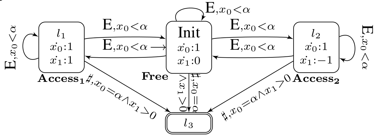
Figure 2 : A Linear Hybrid Automaton (LHA) measuring differences of memory usage File text of this example
To compute the difference of memory usage, Cosmos needs the following HASL formula:
Simulation
To start Cosmos on this example, first go to the directory Examples/SharedMemory from the Cosmos directory, then launch the binary with the following arguments:cosmos sms_Unif.gspn sms_Unif.lha --width 0.01
Those arguments make Cosmos perform simulations until the confidence interval for the HASL formula has a width smaller than 0.01. Cosmos builds an internal representation of the model and the automaton, using code generation, and then starts the simulation.Cosmos:
Start Parsing sms_Unif.gspn
Start Parsing sms_Unif.lha
Parsing OK.
Start building ...
Building OK.
START SIMULATION ...
Estimated value: 0.499119402985075
Confidence interval: [0.494143613790152 , 0.504095192179998]
Width: 0.00995157838984584
Confidence interval computed sequentially using Chows-Robbin algorithm.
Confidence level: 0.99
Total paths: 67000
Accepted paths: 67000
Time for simulation: 5.776912s
Total CPU time: 7.910013
Results are saved in 'Result.res'
The --help option can be used to show the list of available options.Cosmos and the GreatSPN Editor
The Petri net Editor of GreatSPN can be used to design Stochastic Petri Net. The resulting Petri net can be exported to Cosmos using the .GrML file format. Alternatively the editor can start Cosmos and display result of simulation inside its graphical interface.
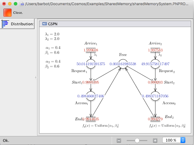
Figure 3 : Screen-shot of the GreatSPN Editor showing results from Cosmos. The red numbers are mean throuput and the blue ones are mean number of tokens.
Cosmos and CosyVerif
Cosmos is integrated inside the CosyVerif platform. This platform provides a graphical front end named Coloane allowing one to draw GSPN and LHA with a graphical editor. Cosmos reads the GRML file format used by CosyVerif, both for GSPN and LHA.
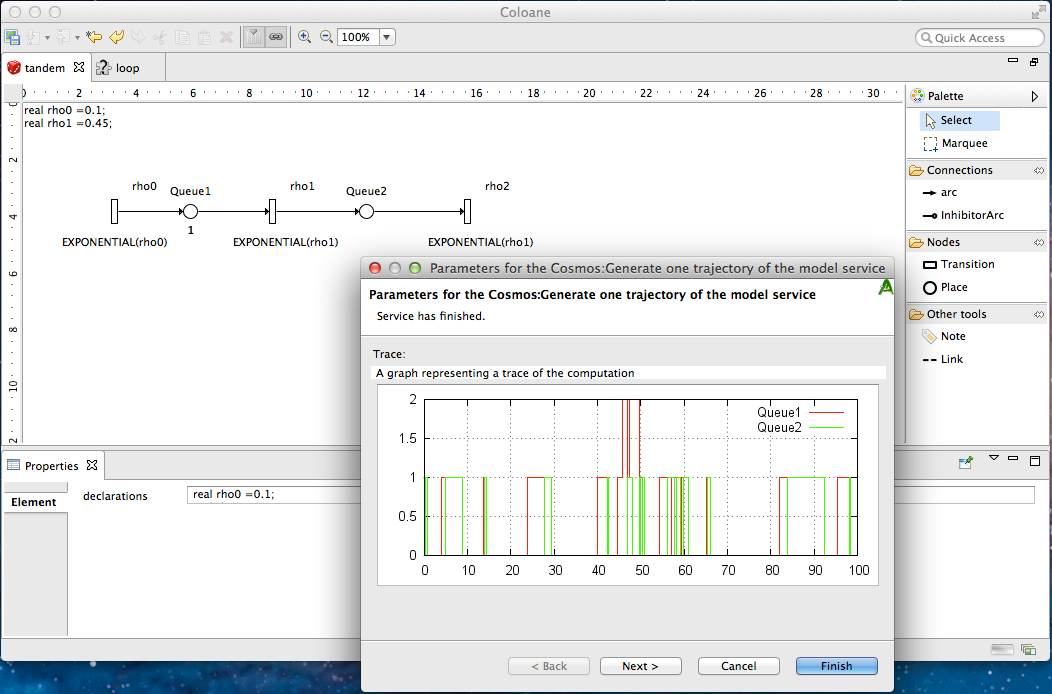
Figure 3 : Screen-shot of the graphical interface of CosyVerif running COSMOS
A complete example
Building a model
▷Download the GreatSPN Editor and start it.
▷Click on the upper left icon to create a new model. The following windows should open:
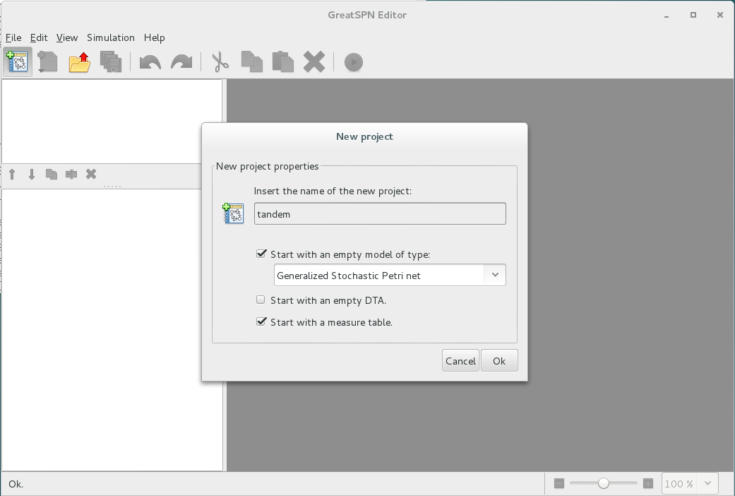
▷ Fill the windows as on the previous screen shoot.
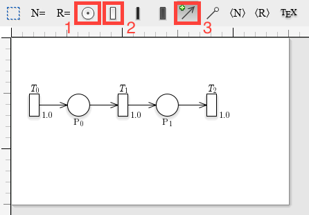
▷ Draw a tandem queues system by adding two places (icon 1), three exponential distributions (icon 2) and adds arc between places and transitions (icon 3) as in the following screenshot:
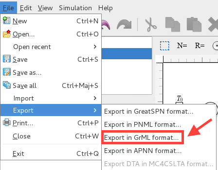
▷Export the model in the GrML file format using the file menu/export/export in GrML.
Simple use of the tool
Cosmos can be used to compute simple performance evaluation indexes of a model by generating an HASL formula. This is done using the ``--loop X'' option which generates a simple LHA which loops for X time units and then accept the trajectory.
▷Open a terminal and go to the directory where you have exported the model.
▷ write down
Cosmos GSPN.grml --loop 100 --width 0.05You should see something similar to the following screenshot:
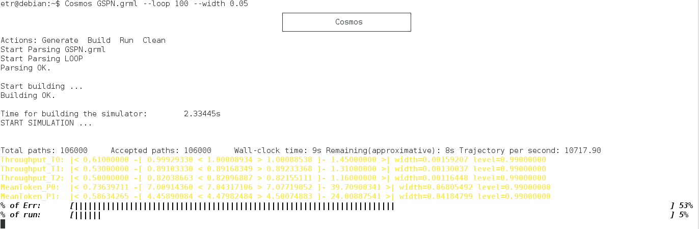
You can observe that Cosmos start by parsing the model and the LHA then the simulator is built and simulations start. Cosmos dynamically updates the state of simulation. The first line in black shows some data on the number of trajectories and simulation time. Each of the following lines (in yellow) is the estimation of an HASL expression. These lines read as follows:
Expr name: |< min value -[ confint low < mean value > confint up -] max value >|Where confint stand for ``confidence interval'' and are followed by the width of the confidence interval and the confidence level used for the confidence interval computation.
The last two lines indicate the progress of the simulation. The first one % of Err: represents the width of the largest confidence interval with respect to the objective (given on the command line with "--width 0.05"). The second line % of run: represents the number of simulated trajectories with respect to the maximum allowed number (by default 2000000). The simulation stop when one of the goals is reached. You can stop the simulation by hitting Ctr-C.
You can plot a single trajectory with the following command
▷Write down the following command line:
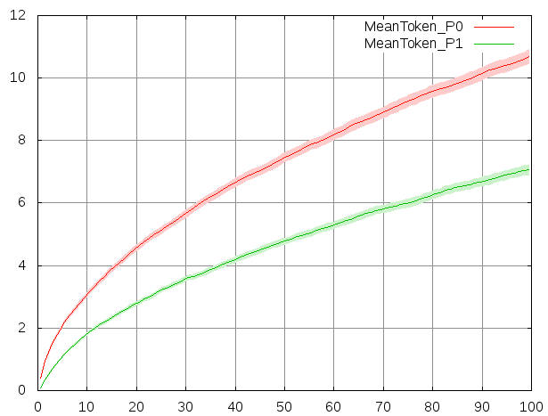
Cosmos GSPN.grml --loop 50 --max-run 1 --output-trace trace.dat 0 --gnuplot-driver pngYou can visualise the behaviours of the model by plotting the mean trajectory.
▷Write down the following command line:
Cosmos GSPN.grml --sampling 100 1 --max-run 100000 --output-graph trace --gnuplot-driver pngThe ``--sampling X Y'' option generate an LHA which samples the value each places each Y time unit and stop the simulation after X time unit. The ``--max-run Z'' option specify the maximal number of runs. The ``--output-graph file'' option output the result of the simulation in the file ``file''. The ``--gnuplot-driver output'' option start the gnuplot software and specify the type of output. At the end of the simulation you can open the file ``trace.png'' which should be similar to this one:
▷Change the rate of transition $T_0$ to $0.6$ in GreatSPN, export the model and run Cosmos, observe the difference of behaviours.
▷Change the type of transition $T_1$ to ``General'' and set the delay to ``I[1.0]'', which stand for Dirac distribution in $1$. Change the sampling parameters to ``--sampling 10 0.1'' to plot a more precise graph.
If a model does not behave as it is intended to, it is useful to perform step by step simulation.
▷ write down the following command line
Cosmos GSPN.grml --loop 100 --output-dot draw.pdf -iCosmos will stop before the first step of simulation and show you the available transitions. You can write down ``s'' to perform one step of simulation, or ``fire Ti'' to fire transition Ti. If you write ``d'' and open the file ``draw.pdf'', it will contain a drawing of the Petri net updated with the current marking.
HASL formula
In this part we will design an LHA to evaluate a more complex property.
You can look at the LHA produced by Cosmos while using options ``--loop'' or ``--sampling''. By default these files are removed with all the temporary files when Cosmos exit. The option ``--tmp-status keep'' prevent Cosmos from cleaning up, all the temporary files are stored in a directory called ``tmp'' in the working directory.
▷Look at the file ``tmp/looplha.lha'' and ``tmp/samplinglha.lha''.
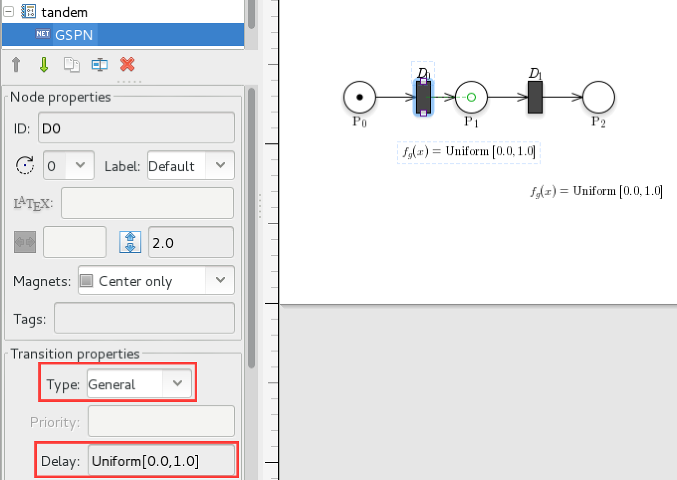
▷ Build a new GSPN in GreatSPN with three places, and two transitions, set the initial marking of the first place to $1$ and $0$ for the others. Add arcs such that the only possible execution is for the token to go from the first place to the second by firing the first transition and then go to the third place by firing the second transition. Then set the distribution of both transitions to be a ``General'' distribution with delay ``Uniform[0.0,1.0]''.
▷ Open a new text file with an ``.lha'' extension with a text editor and write down the following:
VariablesList = {x, y, r} ;
LocationsList = {lx, ly, lf, lp,lm};
%HASH Expression
p=4*PROB;
InitialLocations = {lx};
FinalLocations = {lp};
Locations={
%( location name, guard, flow )
(lx, TRUE , (x:1 , y:0) );
(ly, TRUE , (x:0 , y:1 ));
(lf, TRUE );
(lp, TRUE );
(lm, TRUE );
};
Edges={
%( (source, dest), label, guard, update )
((lx,ly),ALL, # , #);
((ly,lf),ALL, # , {r=x*x + y*y});
((lf,lp), #, r<=1 , #);
((lf,lm), #, r>=1 , #);
};
▷ Can you guess the value of p ?
▷ Run Cosmos by passing the model name and the lha name.
▷ Add an HASL expression to the LHA to compute the mean value of r.
▷ For the tandem queue model, write down an LHA computing the following LTL formula: ``X ( (Q1+Q2>0) U (Q1+Q2=10) )''.