A Sneak Peek at Simulink
Simulink models are a set of boxes connected by wires. Boxes are called Blocks and signals go through wires. Blocks act like operators transforming input signals into output signals. These operators may vary widely in nature:
- Signals may be evaluated in discrete or continuous time;
- There can be a latency introduced by blocks, which can be infinitesimal (i.e. when the block integrates its input signal)
- They may introduce discontinuities to their output signal, for example if its operator includes a test
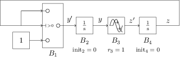
For example, the Switch block B1 checks whether its conditional input is greater than zero; in this case, it outputs the same signal and in the other case, it outputs the constant signal 1. Blocks B2 and B4 are Integrator blocks for which the output signal is the integral of its input signal with the given initial value. Block B3 is a Transport Delay block: it delays the input signal by the given latency.
This already allows to modelize a wide range of differential equations.
Cosmos' Simulink Simulation Engine
Overview
It is easy to generate and use a C code for discrete Simulink models (using only discrete blocks, which are sampled at fixed intervals) using MathWorks tools. However, it limits the expressivity of the models. In order to use more diverse Simulink models and control the flow of a multi-model simulation (with Discrete Event Stochastic Processes) we developed a Simulink Simulation Engine embedded into Cosmos.
Like MATLAB, it computes approximate values for the signals of the model. The Cosmos' Simulink Simulation Engine only supports subset of the Simulink blocks, however large enough to show the main features of Simulink models : threshold crossings (through Switch or Relay (hysteresis) blocks), adaptative Integration methods (through Integrator blocks), latencies (through (Unit) Delay (discrete) and Transport Delay (continuous) blocks).
Sketch of the Cosmos Simulink Simulation loop
We first define a Block Ordering that reflects the dependencies on the computation of signals on a single simulation step. This order is defined as follows: (a.) blocks with no input signals, (b.) blocks with non-infitesimal latency by increasing latency, (c.) infinitesimal latency blocks (Integrators) and (d.) immediate blocks in topological order. Note that if no such topological order exists, there is an immediate dependency loop in the model and it cannot be simulated.
Values of signals will be stored into extensible arrays Bk,o for each output o of each block B of the model. Values of time are stored into an extensible array T. Those are initialized with the (given) initial time tinit, then the values of the blocks are generated using the block ordering. For latencied blocks, we use their initial values.
For each step, we then compute the next simulation time, through sampling times of discrete blocks. It is then refined to respect the precision of the adaptative integration method. Then, if the threshold value of any conditional block is crossed, we compute the threshold crossing time. Once this simulation time is computed, we can then compute the value of every signals processing blocks through the block ordering.
This simulation loop is more thouroughly explained in Integrating Simulink into Cosmos (to appear)
Examples of Simulink models
An exact semantics of Simulink models has also been defined, based on the construction of differential equations through exploration of backwards graphs of Integrator blocks, choice of modes for each conditional block, and instanciation of latency functions which allow to use past behaviour of signals to represent current behaviour of output signals of latency blocks. This allows to check whether results of the simulation engine are approximately correct or not.
Exact semantics of Simulink models are more detailed in Integrating Simulink into Cosmos (to appear)
Running a Simulink model with Cosmos
First, make sure you have an updated version of the OCaml
compiler (at least 4.04) with the following OCaml packages:
zip, xml-light and str. You also need to have compiled
Cosmos. Once these requirements are installed, build the
lastest version of Cosmos' Simulink Simulation Engine using,
from the base folder of Cosmos sources : cd
modelConvert/ then ./build.sh.
Make sure (a.) your model is registered into the .slx format and (b.) the initial simulation time is correctly registered; if necessary, convert the model into this format using Matlab-Simulink.
Once these steps are complete, to simulate a Simulink
model using Cosmos, you need to (a.) compile it
into Cosmos-compatible code using CosmosSimulink
model.slx. It should return a minimal TikZ code that
represents the Simulink model, without any error. If a block
is not recognized, try either modifying the Simulink model
using supported blocks, or contacting the current developer
(Yann Duplouy).
Finally, copy a main.cpp file from any of the Simulink Examples (in Examples/Simulink). You can now call Cosmos:
- using the interactive mode to monitor the
behaviour of the model at each time step,
using
Cosmos SKModel.grml -i; then usesto progress by a single simulation step,w tto compute the model until the time t, andqto interrupt the simulation. - or to process a graph of the
simulation,
Cosmos SKModel.grml --output-trace
              trace.data 0 --gnuplot-driver svg --max-run 1 --loop
              t
where t is the final simulation time.
Switch, Integrators and Delay
Application of exact semantics. We
simulate this model over the time interval [0,2]. Given
the constant zero function for the initial step of
the Transport Delay block
(B3), and the intial conditions of
the Integrator blocks, we know that y(0) =
1 and z(0) = 0.
Over the time
interval [0,1], we are still in the initial condition
of B3, hence z' = 0 which
implies z(t) = 0. The condition
of B1 isn't met, which implies y'
= 1 hence y(t) = t.
The solution over
[0,1] implies that z'(t) = t-1 on the interval
[1,2], which implies, knowing z(1)=0,
that z(t) = (t-1)2/2. The condition
of B1 is now met, which
implies y'(t) = z(t) = (t-1)2/2 and
finally y(t) = (t-1)3/6+1 (because we
had y(1)=1).
Running a Petri net and a Simulink model altogether
Overview
We have implemented a co-simulation loop between slightly enhanced Petri nets and Simulink models into Cosmos. More specifically, we have added two kinds of transitions to Petri nets, which either send new values to the Simulink model or read Simulink signals to generate new bindings for the Petri net.
Example: Double Heater
This example is available inside the source
code of Cosmos, under the folder
Examples/MultiModel/DoubleThermostat. It will be soonly
available on this website in a separate download.
Note: you might currently have to run ./build.sh in the
modelConvert folder of the Cosmos repository (or location)
to have CosmosSimulink properly built and installed before running this example
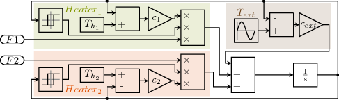
The Simulink model modelises the temperature of a room which is heated by a system of two heaters, each having a different heat diffusion constant ci and a own temperature of Ti. It also modelises the interaction with the external temperature. The model has two inputs, each representing whether a heater is working correctly or out of order.
The two Relay block (with a symbol of hysteresis) controls whether the heaters should be working. In this model, we try to keep the temperature between 20°C and 25°C.
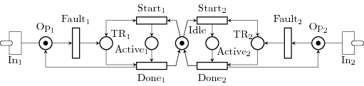
The Petri net both controls the failure rate of each of the heater (with an exponential distribution) and also the behavior of a repairman, which chooses and repair an heater in both a fixed time.
The synchronisation is done through the transitions In1 and In2 which are both synchronisation transitions. They copy the value of Opi (here, a number of tokens) to the signals Hi of the Simulink model.
Note that every synchronisation procedure is encoded into the GSPN model.
In the benchmarkPN18.grml model given in this example, we also read
the temperature given by the Simulink model, through the Synch21O1
transition, connected to the temperature signal.
Running the examples. One can replicate the results presented
in the Integrating Simulink into Cosmos article using both benchmarkPN18.sh
and benchmarkPN18_dti.sh shell scripts. They both consists of two instructions:
- first, compile the Simulink model using
CosmosSimulink. Several options are given. The first,--epsv 0.01is for the precision step of the ODE45 procedure for the Integrator blocks. The second,--skbasestep 1gives the base step (before Integration and Threshold Crossing) of the Simulink model. Finally, the model file is given.
CosmosSimulink --epsv 0.01 --skbasestep 1 benchmarkPN18.slx - second, start Cosmos using first the GRML then the HASL formula you want to check.
Here, we used
--njob 6so Cosmos runs 6 simulations in parallel, and--max-run 500000to precise the number of simulations we want to run.
Cosmos benchmarkPN18.grml benchmarkPN18.lha --njob 6 --max-run 500000